This paper by Olaf Ronneberger, Philipp Fischer, and Thomas Brox from the University of Freiburg, Germany. This architecture was the backbone of the winning solution of the ISBI 2015 cell tracking challenge. Quoting the paper, “Moreover, the network is fast. Segmentation of a 512x512 image takes less than a second on a recent GPU”.

Some Theory

In the Introductory part of the paper, we see the concern that this paper aims to address. Deep Neural networks, that provide state of the art solutions to most visual recognition tasks, they are data-hungry. It requres large numbers of sample training data points to optimize their parameters. Furthermore, we are reminded of the fact that the problem of semantic segmentation and object localization is a more complex problem than image classification.

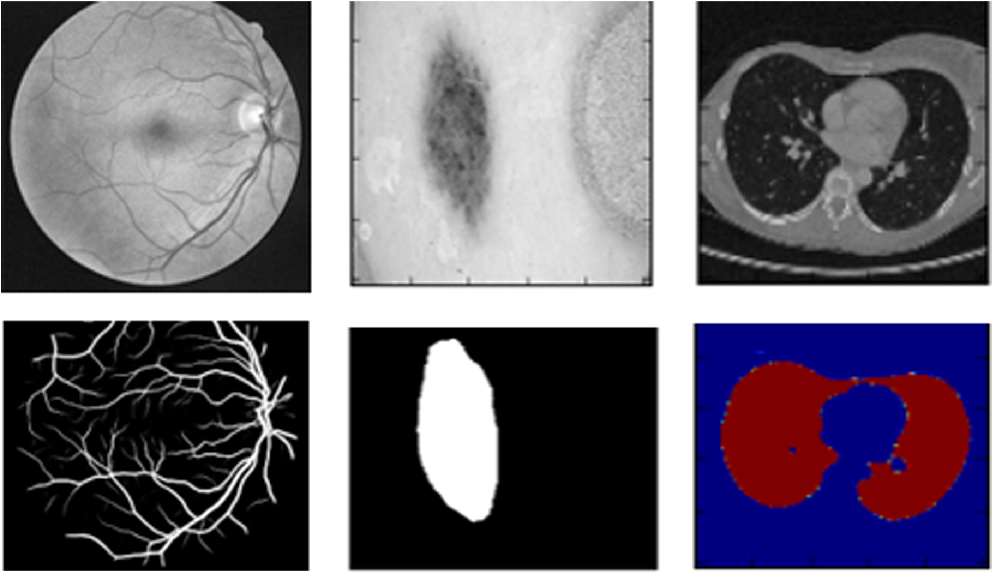
Let us take the example of biomedical image segmentation as shown in the cover of this post. There are several difficulties one faces. Apart from the inherent fact that every pixel must have a label, we are limited in the number of images available in biomedical tasks. Detailed analysis of the paper by Ciresan, D.C., Gambardella, L.M., Giusti, A., Schmidhuber, J.: “Deep neural net-works segment neuronal membranes in electron microscopy images” at NIPS, 2012 that labels each pixel by using a sliding window/ a local patch/ a neighbourhood of the pixel as input. This network localizes well. A significant number of random patches that can be taken is much larger in order than the number of images available and hence we have achieved an augmentation of sorts using such patches. Drawbacks include speed, as for each pixel we have to pass the corresponding patch through the network. The next drawback mentioned needs attention. The size of the patches become a critical choice. Larger patches followed by subsequent maxpooling may abstract the target pixel information compromising localization while smaller patches pass little neighbourhood information to the network. This is the tradeoff between localization accuracy and the use of context.

This paper claims to propose a modified “fully convolutional network”. Let us have a look at the architecture before we describe it.

Previous work on semantic segmentation using Fully convolutional networks include an encoder-decoder architecture (Long, J., Shelhamer, E., Darrell, T.: Fully convolutional networks for semantic segmentation (2014)) where the use of upsampling instead of pooling operations allowed high resolution outputs. For ease of localization high-resolution information from the contracting part is fed to these upsampled outputs followed by a convolution. The intuition is that this convolution may learn a mapping that makes use of the fed high resolution features to improve the segmentation map. In U-NETs a large number of feature channels allow us to propagate a sufficient amount of context information ( what is a pixel with respect to its surroundings?).

The U-Structure is a result of the symmetric contraction and expansion. As we propagate into the depth of any CNN, our field of vision on the input image increases but we may lose localization features and here comes the significance of passing the features from lower depth layers while upsampling for the output. At corner points or boundary regions, we may mirror parts of the input image so as to pass a consistent context. This provides consistency as against zero-padding or other such techniques. This is as shown below

Elastic transformations were used to augment the small data present and thus the network is in variant to such transformed inputs as possibly available at the time of inference.

Note:- Whenever the words constricting, contracting, expanding etc. words are used to describe the architecture, it is to be assumed that we are talking about the image width and height and not the depth of the convolutions.

Architecture and Code

The Constricting part has repeated (3x3 conv - 2x2 maxPool ) units with number of feature channels doubling at each step. The ReLU activation layer is used. The expansive path has the upsampled featured map followed by 2x2 up-convolutions halving the number of feature channels at each step. The symmetrically opposite conv layer in the constricting block feeds its conv features to the corresponding block of the expansive path after upsampling which is followed by another convolution.

Each block of convolution is defined as double convolution before pool as shown in the image. To keep things simple, let’s discuss how this looks in TensorFlow2.0/Keras API. (I personally prefer PyTorch XD)

1
2
3
4
5
6
7
8
9
10
11
12
13
14
15
16
17
18
19
import tensorflow as tf
from tensorflow.keras.layers import *
def conv2d_block(inputs, filters, kernel_size = 3, batchnorm = True):
    """Function to add 2 convolutional layers with the parameters passed to it"""
    # first layer
    x = Conv2D(filters = filters, kernel_size = (kernel_size, kernel_size),\
              kernel_initializer = 'he_normal', padding = 'same')(inputs)
    if batchnorm:
        x = BatchNormalization()(x)
    x = Activation('relu')(x)
    
    # second layer
    x = Conv2D(filters = filters, kernel_size = (kernel_size, kernel_size),\
              kernel_initializer = 'he_normal', padding = 'same')(x)
    if batchnorm:
        x = BatchNormalization()(x)
    x = Activation('relu')(x)
    
    return x

Following this we have to design the constricting and expansive paths in the unet with proper concatenations

1
2
3
4
5
6
7
8
9
10
11
12
13
14
15
16
17
18
19
20
21
22
23
24
25
26
27
28
29
30
31
32
33
34
35
36
37
38
39
40
41
42
43
44
def get_unet(input_img, n_filters = 16, dropout = 0.1, batchnorm = True):
    # Contracting Path
    c1 = conv2d_block(input_img, n_filters * 1, kernel_size = 3, batchnorm = batchnorm)
    p1 = MaxPooling2D((2, 2))(c1)
    p1 = Dropout(dropout)(p1)
    
    c2 = conv2d_block(p1, n_filters * 2, kernel_size = 3, batchnorm = batchnorm)
    p2 = MaxPooling2D((2, 2))(c2)
    p2 = Dropout(dropout)(p2)
    
    c3 = conv2d_block(p2, n_filters * 4, kernel_size = 3, batchnorm = batchnorm)
    p3 = MaxPooling2D((2, 2))(c3)
    p3 = Dropout(dropout)(p3)
    
    c4 = conv2d_block(p3, n_filters * 8, kernel_size = 3, batchnorm = batchnorm)
    p4 = MaxPooling2D((2, 2))(c4)
    p4 = Dropout(dropout)(p4)
    
    c5 = conv2d_block(p4, n_filters = n_filters * 16, kernel_size = 3, batchnorm = batchnorm)
    
    # Expansive Path
    u6 = Conv2DTranspose(n_filters * 8, (3, 3), strides = (2, 2), padding = 'same')(c5)
    u6 = concatenate([u6, c4])  #Note the concatenation after the upsampling
    u6 = Dropout(dropout)(u6)
    c6 = conv2d_block(u6, n_filters * 8, kernel_size = 3, batchnorm = batchnorm)
    
    u7 = Conv2DTranspose(n_filters * 4, (3, 3), strides = (2, 2), padding = 'same')(c6)
    u7 = concatenate([u7, c3])
    u7 = Dropout(dropout)(u7)
    c7 = conv2d_block(u7, n_filters * 4, kernel_size = 3, batchnorm = batchnorm)
    
    u8 = Conv2DTranspose(n_filters * 2, (3, 3), strides = (2, 2), padding = 'same')(c7)
    u8 = concatenate([u8, c2])
    u8 = Dropout(dropout)(u8)
    c8 = conv2d_block(u8, n_filters * 2, kernel_size = 3, batchnorm = batchnorm)
    
    u9 = Conv2DTranspose(n_filters * 1, (3, 3), strides = (2, 2), padding = 'same')(c8)
    u9 = concatenate([u9, c1])
    u9 = Dropout(dropout)(u9)
    c9 = conv2d_block(u9, n_filters * 1, kernel_size = 3, batchnorm = batchnorm)
    
    outputs = Conv2D(1, (1, 1), activation='sigmoid')(c9) # the 1x1 Conv 
    model = Model(inputs=[input_img], outputs=[outputs])
    return model

Note: If the sizes are incompatible for concatenation we need to crop before we concatenate

Training

The model is trained end to end as a supervised model with the input images and the corresponding segmentation maps. Use of large tiles as input is recommended so as to minimize the GPU overhead. This can be achieved by compromising the batch size. At the time of inference, batch size will be low but these large tiles will allow minimum execution time. A momentum-based optimizer like Adam may be used but the paper uses SDG with momentum 0.99 arguing that such a high momentum allows previous examples to further impact the current optimization step thereby taking a more general step in our optimization space. They used a softmax function followed by a cross entropy evaluation. The softmax function is ${p}_k(\vec{x}) = {\exp({a_k(\vec{x})}) \over \left(\sum_{k' = 1}^K \exp(a_{k'}(\vec{x}))\right)}$ where \(a_k(\vec(x))\) is the activation of the last layer ie. the 1x1 Conv layer. This Softmax activation converts the ouput vector into probabilities and the elements of the obtained vector adds up to 1 along the dimension in which softmax is applied. Let us have a look at the cross entropy function as shown in the paper

where \( \ell:\Omega \rightarrow {1,\dots,K} \) is the true label of each pixel and \( w:\Omega \rightarrow \mathbb{R} \) is a weight map that they introduced to give some pixels more importance in the training.

Let us try and understand why cross entropy was used in the first place. Any segmentation map, as seen in the cover picture has labels its pixels into one of a finite set of classes. For Eg, lets have a look at the following segmentation map.

Each pixel of the segmentation map may be one of four classes(black, blue, green or red). Entropy as shown in \( \ref{eq1} \) quantifies the uncertainty in a vector. It is maximum when all events are equiprobable and zero when one event is certain and the remaining are zero (In our case, the exact nature of the pixel is certain).

\( w:\Omega \rightarrow \mathbb{R} \) is a weight map introduced in the paper. There is an inherent need to give some pixels more importance than others in medical image analysis. For eg. Tumor cells may be more important to be correctly segmented than healthy cells as we definitely do not want to label a sick patient healthy. Additionally such a weight map must also deal with the class imbalances as the healthy cells are much more in number than the unhealthy ones.

Lets have the formal definition of the weight map from the paper after evaluation of the seperation borders from morphological operations:

$\begin{equation} \label{weightmap} w(\vec{x}) = w_c(\vec{x}) + w_0 \cdot \exp\left( - \frac{(d_1(\vec{x}) + d_2(\vec{x}))^2}{2\sigma^2}\right ) \end{equation}$ where $w_c:\Omega \rightarrow \mathbb{R}$ is the weight map to balance the class frequencies, $d_1:\Omega \rightarrow \mathbb{R}$ denotes the distance to the border of the nearest cell and $d_2:\Omega \rightarrow \mathbb{R}$ the distance to the border of the second nearest cell. In their experiments they set $w_0 = 10$ and $ \sigma \approx 5 $ pixels.

The weights of the architecture overall, are initialized as sampled from “Gaussian Distributions with a standard deviation of $\sqrt{2/N}$, where $N$ denotes the number of incoming nodes of one neuron”.

Thus we have the definition of the model, the proper weights initialization, a clear understanding of the loss used and its quantification of the uncertainty in the discrete classes as seen in the segmentation maps.

Do go ahead and read the paper and compare the inferences made in the blog with your intuitions.