The curves given above are known as Gaussians. This post aims to discuss what they are, what they mean and to gain intuitive intuitions into what they signify. We shall further learn to hallucinate sample points from such curves and look at what likelihood means. These concepts are fundamental to machine learning and statistics in general.

Networks such as Generative Adversarial Networks(GANs) depend on these fundamental concepts and one shouldn’t dive into such networks without first understanding these concepts and gain an insight into randomness and information.

Let’s first simply look at Gaussians as a curve in mathematics, and then we will try to come to the concept of it being a probability distribution and infer what that means. The equation goes as follows :

$$\begin{equation} \label{GaussianEq} p(x) = {1 \over \sqrt{2\pi\sigma^2}} \hspace{0.1cm} e^{- {1 \over 2 \sigma^2}(x - \mu)^2} \end{equation}$$

where \( \mu \)= mean of all values of x and \(\sigma \)= the standard variance of all values of x. We shall show these later

Let us have a look at this curve and draw inferences on its nature.

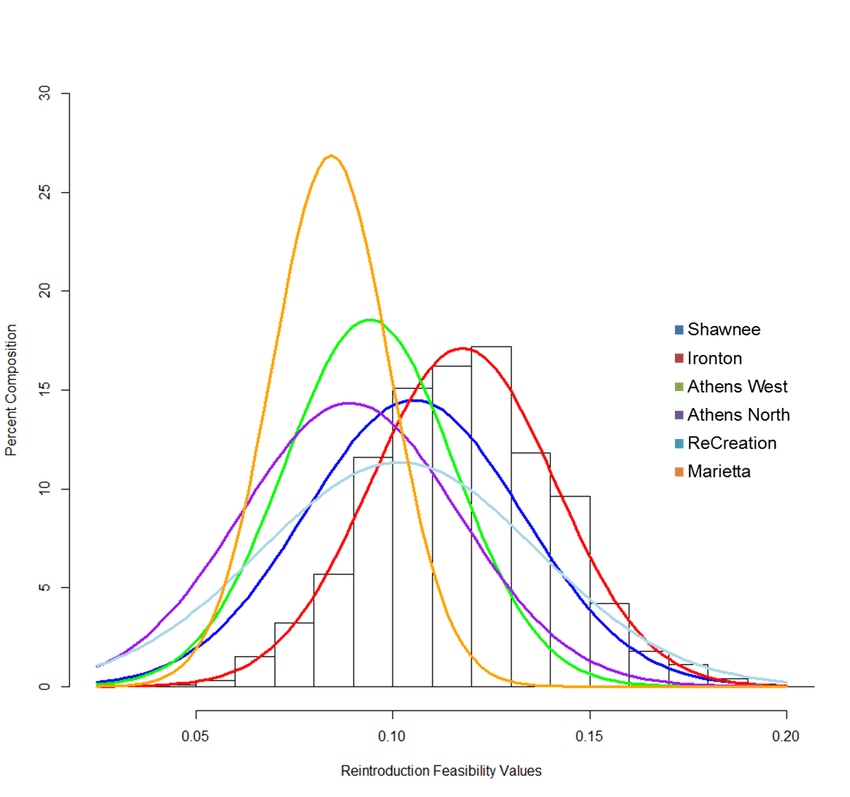
The highest point of this curve corresponds to \( x = \mu \) . We have taken a special case where \( \mu = 0 \) and \( \sigma = 1 \). In such a case, these are known as normalized Gaussians. Notice the cover figure of the post, the position of the different peaks are the means of those curves. \( \sigma \) tells us distribuited the data is away from the mean. So, the more spread out the curve, the higher is the value of \( \sigma \).

Note that $\int_{-\infty}^{+\infty} p(x) dx = 1$. This means that the fucntion is a Probability Distribution Function. If we have a set of values of x that are Gaussian distributed, ie $\textbf{x} : \{x_1, x_2, x_3, \dots\}$ , then we mean to say that their occurence that a sample from x being some \( x_k\) follows the probability as per the curve depeinding on them mean of x \( \mu_x \) and the standard deviation \( \sigma_x \). \( \mu \) and \( \sigma \) are the only two parameters needed to get this distribution and hence they are together referred to as the sufficient statistics.

Looking at Machine learning from this point of view, we are all looking to develop models that find the “sufficient statistics” for realizing a function.

Simulation or Hallucination

From what has already been discussed, we should be able to infer the meaning of a distribution and its points. But, quite often in machine learning, we have to sample values from a given Gaussian distribution to get an array of certain dimensions. Eg: make an array of 100 numbers such that they are from the Gaussian given by mean=0 and standard deviation=0.2. This process of sampling is called Simulation or Hallucination.

It may be denoted as $\textbf{x} \sim N(\mu, \sigma^2)$. To Understand this let us look as the Cumulative Distribution function which is as shown :

$$\begin{equation} \label{CDF} F(x) = P(X \leq x) = \int_{-\infty}^{x} p(u) du \end{equation}$$

Graphically,

To sample from the Gaussian distribution, we will use the PDF, CDF and a random number generator(RNG). RNG functions are implemented in all popular programming languages. We will use a random number geneator $rng(x) \in [0,1]$. This follows a uniform distribution and all values are equiprobable.

Let us now have a look at the process.

For a single output of the RNG, say 0.65, we would project it on to the CDF and take the corresponding value of $x$. Notice how a large portion of the rng numbers would project itself onto the linear section of the graph and thus be closer to the mean, as controlled by the variance. We are consistent with our PDF in this approach.

Expectation , Monte Carlo convergence and a reference to Information

The Expectation of a PDF refers to the most likely result of a single simulation of a PDF. For Gaussian distributions, this is easily visualizable from the graph that the mean is the expected value. if we encounter any random variable x, it is by the expectation that we define the mean.

$$\begin{equation} \label{expectation} \mathbb{E}(x) = \int_{-\infty}^{x} x p(x) dx = \mu = {1 \over N} \Sigma_{i=1}^N X^{(i)} \end{equation}$$

The second equality to the summation os only valid for large values of $N$ in which case the sum converges to the integral for random variables. This is known as the Monte Carlo convergence.

Gaussians also have importance from the perspective of adding information to models. In the frequency domain, Gaussians are just a line parallel to the X-axis and are familiar to communication Engineers as AWGN. It does not discriminate but adds equally with all frequency components of a signal. Thus, in Generative models, the use of Gaussians further indicates the addition of the minimum possible bias to the model. This is further supported by the Central Limit Theorem according to which as the number of independent random variables added together tend to infinity, their distribution approaches a Gaussian.

Covariance and multivariate Gaussians

Covariance of two R.Vs X and Y tell us to what extent X and Y are Linearly related.

$$\begin{equation} \label{covariance} cov[X,Y] = \mathbb{E}[(X- \mathbb{E}[X])(Y- \mathbb{E}[Y]) = \mathbb{E}[XY]-\mathbb{E}[X]\mathbb{E}[Y] \end{equation}$$

Note : $cov[X,X] = Var[X] = \sigma^2(X)$ and $cov[X,Y] = cov[Y,X]$

The covariance matrix of a d-length vector $\textbf{X}$ where each feature is a random variable, on the other hand gives us an idea of how each feature is related with respect to the others. ie. for $\textbf{X} = (x_1, x_2, x_3, \dots , x_d)$ where each $x_k$ is a random variable, The covariance matrix is as shown,

$$\begin{equation*} \label{covmat} COV [X] = \begin{pmatrix} VAR[x_1] & COV[x_1, x_2] & COV[x_1, x_3] & \ldots & COV[x_1, x_d] \\ COV[x_2, x_1] & VAR[x_2] & COV[x_2, x_3] & \ldots & COV[x_2, x_d] \\ \vdots & \vdots & \vdots & \ldots & \vdots \\ COV[x_d, x_1] & COV[x_d, x_2] & COV[x_d, x_2] &\ldots & VAR[x_d] \end{pmatrix} \end{equation*}$$

It is denoted by $\Sigma$. This matrix is symmetric in nature and knowing the upper triangular part or the lower triangular part would be sufficient to replicate the matrix entirely.

Let us define the multivariate Gaussian here and then go into a sanity or validity check. This is the gaussian function in higher dimensions (say d dimensions):

$$\begin{equation} \label{multivarate_gaussian} N(X | \mu, \Sigma) := {1 \over {(2\pi)}^{d\over 2} {|\Sigma|}^{1 \over 2}} e ^{-{1 \over 2}(X - \mu)^T \Sigma^{-1}(X - \mu) } \end{equation}$$

$\textbf{X} = (x_1, x_2, x_3, \dots , x_d)$ where each $x_k$ is a random variable and $\mu = (\mu_1, \mu_2, \mu_3, \dots , \mu_d)$

To make sure that we have grasped the concept of sufficient statistics and a multivariate distribution, Let us take up $X = (X_1, X_2)$ where $X_1, X_2$ are two random variables with means $\mu = (\mu_1,\mu_2)$ but having the same variance.

$x_1 \sim N(\mu_1, \sigma^2)$, $x_2 \sim N(\mu_2, \sigma^2)$ where $x_1$ and $x_2$ are samples from $X_1$ and $X_2$.

We need the means and the covariance matrix as sufficient statistics.

1. $(\mu_1,\mu_2)$ : 2 parameters
2. $COV [X] = \begin{pmatrix} VAR[x_1] & COV[x_1, X_2] \\ COV[x_2, x_1] & VAR[x_2] \end{pmatrix}$ .

Since this matrix is symmetric, we only need one of $COV[x_1, x_2]$ or $COV[x_2, x_1]$: 3 parameters

So number of sufficient statistics is : 5.

Let us use this 2D distribution to have a look at the joint probability distribution. That is the probability of a sample of $x_1$ and a sample of $x_2$ occuring at the same time.

Let’s define the matrix notations. $X$ and $\mu$ are column vectors.

$$X - \mu = \begin{pmatrix} x_1 - \mu_1 \\ x_2 - \mu_2 \end{pmatrix}$$ $$\Sigma = \begin{pmatrix} VAR[x_1] & COV[x_1, x_2] \\ COV[x_2, x_1] & VAR[x_2] \end{pmatrix}$$

If $x_1$ and $x_2$ are independent their covariance is $0$.

$$\therefore \Sigma = \begin{pmatrix}\sigma^2 & 0 \\ 0 & \sigma^2 \end{pmatrix}$$

Let’s have a look at the determinant.

$$\begin{align*} |\Sigma| &= \begin{vmatrix} \sigma^2 & 0 \\ 0 & \sigma^2 \end{vmatrix}\\ &= \sigma^4 \end{align*}$$ $$\begin{equation} \therefore \sigma^2=|\Sigma|^{1 \over 2} \end{equation}$$

Now let’s explot the independence of $x_1$ and $x_2$ meaning

$$\begin{align*} P(x_2 | x_1) &= P(x_2)\\ \therefore P(x_1,x_2) &= P(x_2 | x_1) P(x_1) \\ &= P(x_2) * P(x_1) \\ &= {1 \over \sqrt{2\pi\sigma^2}}e^{-{1 \over {2\sigma^2}}(x_2 - \mu_1)^2} * {1 \over \sqrt{2\pi\sigma^2}}e^{-{1 \over {2\sigma^2}}(x_2 - \mu_2)^2} \\ &= {1 \over 2\pi|\Sigma|^{1 \over 2}}e^{(-{1 \over 2}[(x_1 - \mu_1)(x_2 - \mu_2)] \begin{pmatrix}\sigma^2 & 0 \\ 0 & \sigma^2 \end{pmatrix}^{-1} \begin{pmatrix}x_1 - \mu_1 \\ x_2 - \mu_2 \end{pmatrix})} \\ &= {1 \over {(2\pi)}^{d\over 2} {|\Sigma|}^{1 \over 2}} e ^{-{1 \over 2}(X - \mu)^T \Sigma^{-1}(X - \mu) } \end{align*}$$ $$\begin{equation} \label{final} \therefore P(x_1,x_2)={1 \over {(2\pi)}^{d\over 2} {|\Sigma|}^{1 \over 2}} e ^{-{1 \over 2}(X - \mu)^T \Sigma^{-1}(X - \mu) } \end{equation}$$

We see that \ref{final} is the same as the expression for multivariate Gaussians. This fundamental understanding is crucial to grasping the concepts of likelihood and Maximum Likelihood Estimation which shall be the next post in this Basics section.